LP Replication

Linear Local Projections in R example

Author

Andro Asatashvili

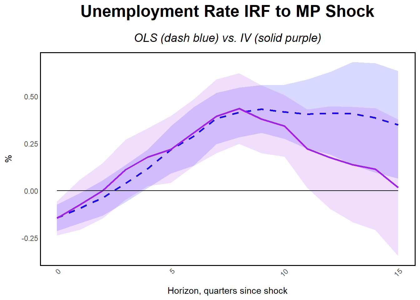
Replication of Local Projections with Instrumental Variable. The Romer and Romer shock (2004) is utilized to construct impulse response functions to see OLS and IV estimation of the unemployment rate to a monetary shock. The instrument seeks to solve the contaminated forward-looking Federal Reserve behaviour and endogenity issues present in the linear case.

Please check the paper!

Local Projections (LP) have the following form:

\[ y_{t+h} = \alpha_{h} + \beta_{h} \Delta r_{t} + \gamma_{h} x_{t}' + {u}_{t+h}, \hspace{10mm} h =0,1,...,H \]

where \(\alpha_{h}\) is an intercept, \({\beta}_{h}\) are our parameters of interest, \(\gamma_{h}\) are estimated parameters for control variables \(x_{t}'\) and \({u}_{t+h}\) are autocorrelated/heteroskedastic disturbances. \(\beta_{h}\) can be interpreted as the impulse responses of \(y_{t+h}\) to a reduced form shock in \(t\). Specificaly, \(\mathcal{R}_{\Delta r \rightarrow y}(h) = \beta_h\). Its common to use Newey and West standard errors due to the serial correlation of \(u_{t+h}\).

In this context, \(y_{t+h}\) is the unemployment rate and \(\Delta r_{t}\) is the Federal Funds Rate. If \(\Delta r_{t}\) is not exogenously determined but we have \(z_t\) available as an instrument, we can then estimate the LP using instrumental variable methods.

To delve deeper and accurately into these methods, please check Jordá (2005) for Local Projections and Stock and Watson (2017) for LP-IV.

Packages

rm(list = ls())

library(foreign)
library(plotly)
library(dplyr)
library(zoo)
library(sandwich)
library(lmtest)
library(AER)
library(ggplot2)
library(haven)
library(dynlm)
library(downloadthis)

Data

Where UNRATE is the unemployment rate, DFF is the Federal Funds Rate. The resid variables are the Romer and Romer shock.

data <- read_dta("RR_monetary_shock_quarterly.dta")
lpiv <- read_dta("lpiv_15Mar2022.dta")

data <- merge(data, lpiv, by = "date", all.x = TRUE)
data <- data %>%
  select(-date)

data <- data[!is.na(data$resid_full), ]
head(data)

1: Data available on Òscar Jordá’s website
2: Keep only nonmissing observations in resid_full

        resid resid_romer  resid_full   UNRATE      DFF
1 -0.24526549 -0.24604897 -0.22740914 3.400000 6.567444
2  0.58851657  0.59067453  0.67491876 3.433333 8.332527
3  0.51913821  0.51929798  0.48436265 3.566667 8.981087
4  0.14714671  0.14791178  0.16585590 3.566667 8.941630
5 -0.65963701 -0.66056323 -0.57453706 4.166667 8.558889
6 -0.02406602 -0.02591258 -0.02597183 4.766667 7.883297

start_date <- as.yearqtr("1969 Q1", format = "%Y Q%q")
end_date <- as.yearqtr("2007 Q4", format = "%Y Q%q")
date_seq <- seq(start_date, end_date, by = 0.25)

date_data <- data.frame(date = date_seq)
data <- cbind(data, date_data)

hmax <- 16

3: by = 0.25 for quarters
4: Horizon: 16 quarters = 4 years after shock

Local Projection

I’m assuming the variables are stationary. We control for 4 lags of the Federal Funds Rate and 4 lags of the Unemployment Rate itself.

# Generate LHS variables for the LPs
for (h in 0:hmax) {
  data[[paste0("ur", h)]] <- lead(data$UNRATE, h)
}

# LP-OLS
b_ls <- rep(0, hmax)  # Betas
u_ls <- rep(0, hmax)  # Upper bound CI
d_ls <- rep(0, hmax)  # Lower bound CI

for (h in 0:hmax) {
  formula_str <- as.formula(paste0("ur", h, " ~ DFF + lag(DFF,1) + lag(DFF,2) + lag(DFF,3) + lag(DFF,4) + 
                                   lag(UNRATE, 1) + lag(UNRATE, 2) + lag(UNRATE, 3) + lag(UNRATE, 4)"))
  model <- lm(formula_str, data = data)
  coeftest_model <- coeftest(model, vcov = NeweyWest(model, lag = h))
  
  b_ls[h] <- coef(coeftest_model)["DFF"]
  u_ls[h] <- confint(coeftest_model, parm = "DFF", level = 0.90)[,2]
  d_ls[h] <- confint(coeftest_model, parm = "DFF", level = 0.90)[,1]
}

# LP-IV
b_iv <- rep(0, hmax)  # Betas
u_iv <- rep(0, hmax)  # Upper bound CI
d_iv <- rep(0, hmax)  # Lower bound CI

# IV regression using instrument 'resid_full'
for (h in 0:hmax) {
  formula_str <- as.formula(paste0("ur", h, " ~ DFF + lag(DFF,1) + lag(DFF,2) + lag(DFF,3) + lag(DFF,4) + 
                                   lag(UNRATE, 1) + lag(UNRATE, 2) + lag(UNRATE, 3) + lag(UNRATE, 4) |
                                   lag(DFF, 1) + lag(DFF, 2) + lag(DFF, 3) + lag(DFF, 4) + 
                                   lag(UNRATE, 1) + lag(UNRATE, 2) + lag(UNRATE, 3) + lag(UNRATE, 4) +
                                   resid_full"))
  model_iv <- ivreg(formula_str, data = data)
  coeftest_model_iv <- coeftest(model_iv, vcov = NeweyWest(model_iv, lag = h))
  
  b_iv[h] <- coef(coeftest_model_iv)["DFF"]
  u_iv[h] <- confint(coeftest_model_iv, parm = "DFF", level = 0.90)[,2] 
  d_iv[h] <- confint(coeftest_model_iv, parm = "DFF", level = 0.90)[,1]
}

# Create data frame for plotting
plot_data <- data.frame(
  Quarters = 0:(hmax - 1),
  b_ls = b_ls,
  u_ls = u_ls,
  d_ls = d_ls,
  b_iv = b_iv,
  u_iv = u_iv,
  d_iv = d_iv
)

ggplot(plot_data, aes(x = Quarters)) +
  geom_ribbon(aes(ymin = d_ls, ymax = u_ls), fill = "blue", alpha = 0.15) +
  geom_line(aes(y = b_ls), color = "blue", linetype = "dashed", size = 1) +
  geom_ribbon(aes(ymin = d_iv, ymax = u_iv), fill = "purple", alpha = 0.15) +
  geom_line(aes(y = b_iv), color = "purple", size = 1) +
  geom_line(aes(y = 0), color = "black") +
  labs(
    title = "Unemployment Rate IRF to MP Shock",
    subtitle = "OLS (dash blue) vs. IV (solid purple)",
    y = "%",
    x = "Horizon, quarters since shock"
  ) +
  theme_minimal() +  
  theme(
    plot.title = element_text(hjust = 0.5, size = 20, face = "bold"),  # Center the title
    plot.subtitle = element_text(hjust = 0.5, size = 14, face = "italic", margin = margin(t = 10, b = 10)),  
    axis.text.x = element_text(angle = 45, hjust = 1),  # Rotate x-axis labels
    panel.grid.major = element_blank(),  # Remove major grid lines
    panel.grid.minor = element_blank(),  # Remove minor grid lines
    panel.border = element_rect(color = "black", fill = NA, size = 1),  # Add black box around the graph
    axis.line = element_blank(),  # Remove axis lines to place axes outside the box
    axis.ticks.length = unit(-0.25, "cm"),  # Adjust tick lengths to move labels outside the box
    axis.title.x = element_text(margin = margin(t = 10)),  # Adjust margin for x-axis title
    axis.title.y = element_text(margin = margin(r = 10)),  # Adjust margin for y-axis title
    legend.position = "top",  # Place legend at the top
    legend.title = element_blank(),  # Remove legend title
    legend.text = element_text(size = 12)
)

5: Newey and West Standard Error
6: We use a 90% CI